
On this page
Most of what I have written on this blog is about artificial neural networks. Layers, losses, optimizers. And for a long time that was enough. Then one day I realised I could train a transformer but could not explain why an actual neuron fires. The word “neuron” in my own code was borrowed, and I had never looked at where it came from.
So I gave myself a project. Learn computational neuroscience properly, and do it the only way that sticks for me: by building every model, breaking it, and checking whether I understood it.
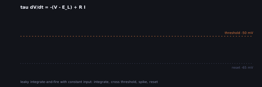
That little trace is where everything started. It is the leaky integrate-and-fire neuron: the voltage charges up like a leaky capacitor, hits a threshold, fires, and resets. It is almost embarrassingly simple, and I still came back to it more than to any other model.
Eighteen weeks, on purpose
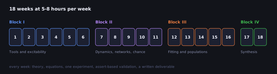
I wanted a plan I could actually finish next to a full-time job, so I settled on 18 weeks of 5-8 hours each. The first block is about single neurons (LIF, Hodgkin-Huxley, synapses). The second moves to dynamics and networks: fixed points, populations that oscillate, Hopfield memories, noisy spike trains. The third is about fitting models to data, and the last one is a specialization and a capstone.
Most of the material comes from the Neuromatch Academy curriculum, which is free and excellent. My roadmap only links to it; the code and the notebooks are my own take on each topic.
The figures that lied to me
Every week ends in the same way: a Python script that runs one experiment, draws a figure, and
then checks the result with a few asserts. The notebook you see on GitHub is generated from that
script, so there is only one source to keep up to date, and a test fails if they drift apart.
The checks felt like overkill at first. They stopped feeling that way quickly.
In week 4 I blocked the potassium channels of a Hodgkin-Huxley neuron to see what happens to the action potential. The plot showed a big swing of voltage right at the start, before any stimulus, and for a while I tried to explain it as biology. It was not. I was starting the simulation at -65 mV, a resting potential that simply does not exist once potassium is gone; the real equilibrium sits above -20 mV. The neuron was just falling towards it. In week 13 the text claimed standard errors for a Poisson model that the code never computed. Both looked perfectly reasonable on the page.
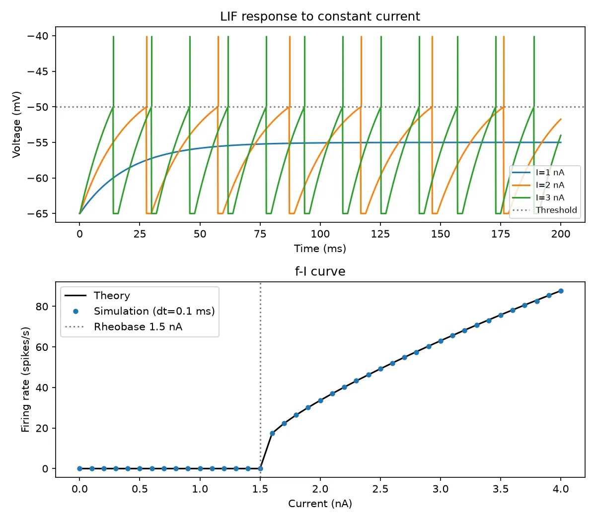
Week 3 is my favourite kind of check. The simulated firing rate has to land on the analytic f-I curve, point by point, and nothing fires below the 1.5 nA rheobase:
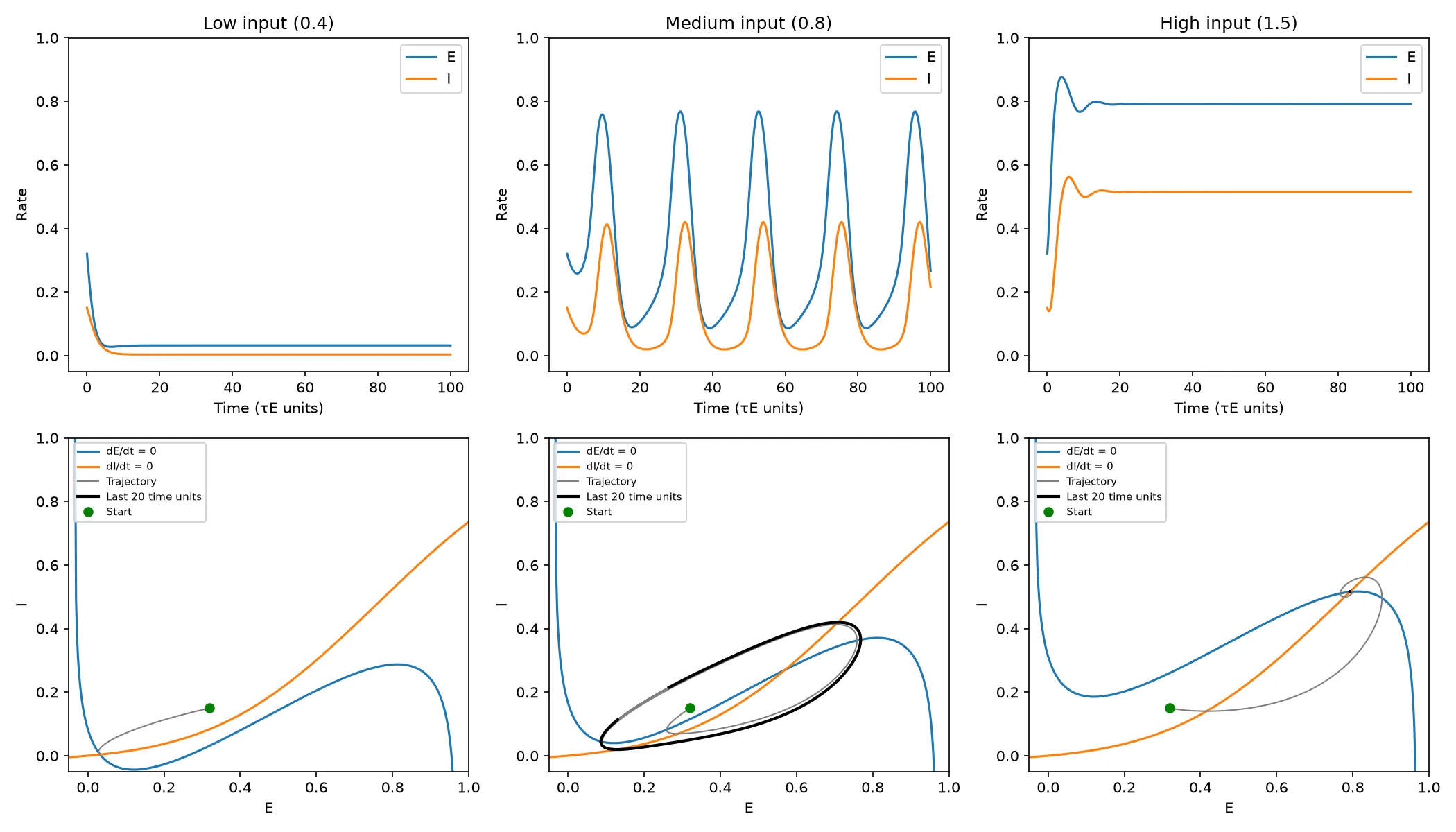
And week 8 is where dynamics finally clicked for me. Same Wilson-Cowan circuit, same connections; only the input changes, and the populations go quiet, start oscillating, or saturate:
Sliders beat paragraphs
Reading that a system “undergoes a Hopf bifurcation” did very little for me. Dragging a slider until a fixed point turns into an orbit did a lot. So the key models also got their own page: plain HTML and JavaScript, nothing to install, and they work on a phone.
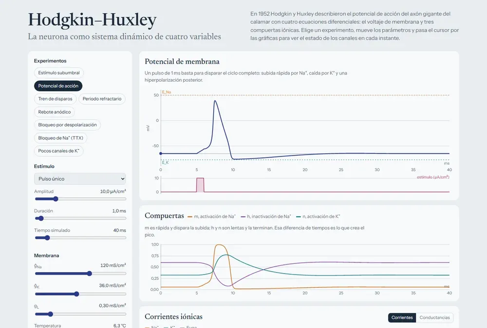
There are nine of them now:
| Module | What I use it for |
|---|---|
| LIF neuron | Watching noise turn regular firing into irregular firing |
| Hodgkin-Huxley | Seeing which gate does what during a spike |
| Synapses | How close two inputs must be to add up |
| 2D linear systems | Clicking around the trace-determinant plane |
| Wilson-Cowan | Finding the input where oscillations begin |
| Hopfield network | Corrupting a memory and watching it come back |
| Poisson spike trains | How a refractory period changes “random” |
| Bayesian decision | Moving the prior and the decision boundary |
| fNIRS with real data | The one below |
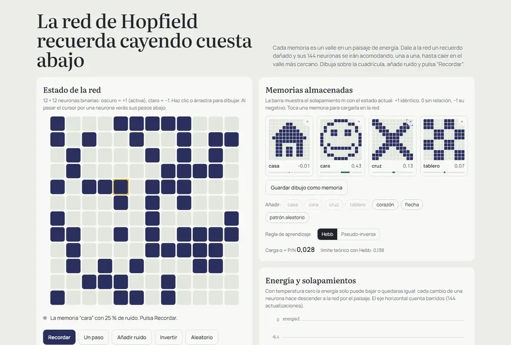
Making them work on a phone was more annoying than building them. The charts looked stretched on my phone because every redraw scaled the canvas by the pixel ratio one more time. And I could not even test a real phone width on my laptop, because Windows will not let a browser window get much narrower than 500 px, so I ended up checking each page inside a 390 px frame.
Then I wanted real data
Simulations only take you so far. At some point you want to see a signal that came out of an actual head. I found Cedalion, a Python framework for fNIRS, which measures changes in blood oxygenation through the scalp with near-infrared light. Its tutorial uses a classic experiment: tap the fingers of one hand, and the motor cortex on the opposite side should get more oxygenated blood.
I analysed one subject in a notebook, using the first 1000 seconds of the recording, 8 trials per hand. (With the full recording the model fit took over half an hour, which is too long for something I wanted to rerun often.)
The left hand worked beautifully. Twelve channels showed a significant increase in oxygenated hemoglobin, and 11 of them were on the right hemisphere, exactly where they should be. The strongest one peaked around 8 seconds after tapping started, and a plain block average without any model matched the fitted response with r = 0.88. The right hand pointed the same way, but no channel survived the correction for multiple comparisons. With 8 trials, I am leaving that one open.
The part I learned the most from was a mistake I almost kept. The original tutorial compares tapping against a “Control” condition, and I did the same. The right hand came out bilateral, which made no sense. Looking closer, the Control condition itself was lowering oxygenation in 10 channels, so subtracting it painted those drops as activations. Comparing against rest instead made the pattern disappear. I had treated the choice of baseline as a coding detail, and it was really part of the question I was asking.
A license I almost missed
When I wanted to put this data in a public demo, I read the dataset’s README properly:
Please use only for Cedalion example notebooks. No other use permitted.
So the notebook downloads that data when it runs, and the repository never ships it. For the demo I switched to an open dataset, fNIRS Finger Tapping Data in BIDS Format by Robert Luke and David McAlpine, with 5 subjects and 30 trials per condition. A script runs the same analysis on all of them in about 18 minutes and writes the results into a file the page loads directly.
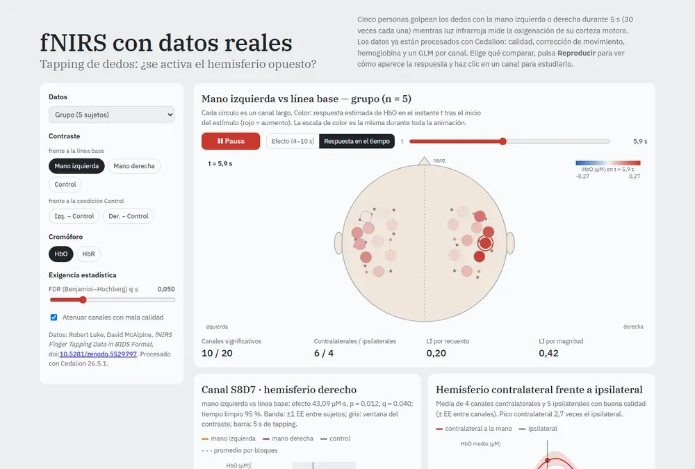
You can pick a subject or the group average and press play to watch the response build up over the motor cortex and fade after the 10 seconds of tapping. Lateralization comes out contralateral in 9 of the 10 subject-hand combinations, which was a relief after the single-subject drama.
Where it stands
All 18 weeks have their script and notebook, each one validated. The nine demos are online. The fNIRS extension has its notebook and its demo. Synaptic plasticity and reinforcement learning are still missing, and they are next on the list. The code is MIT licensed, and every dataset keeps its own terms.
None of this replaces a real course or the papers, and the fNIRS part is for learning, not for anything clinical. But I have something now that I did not have when I started: for every model in the roadmap, I can guess what a parameter change will do, run it, and find out whether I was right. Usually I am not, and that is the useful part.
If you want to poke at it:
- Code and notebooks: github.com/HiroForYou/computational-neuroscience
- Interactive modules: hiroforyou.github.io/computational-neuroscience/interactive
- The Cedalion tutorial paper: Middell, E. et al. (2026), Neurophotonics 13(S3), S32602, doi:10.1117/1.NPh.13.S3.S32602
Comments